Treating Image Edges

There are some good examples floating around of creating customized image processing kernels in the python imaging library (PIL). It's very convenient to simply define your own mask, and the library takes care of the convolution.

One drawback is that the edges don't get filtered in this process. There are various ad-hoc things you can do. You can just drop a line of pixels all the way around the picture, so the gradient image of a 800x600 picture would be 798x598 pixels (if you're using a compact stencil), or you could just copy the edge pixels from the old picture to the new picture. So in effect, the edges don't get filtered. For most applications this is probably no big deal, but it might be, and we can do better.

All we have to do is change our difference operator for the edge pixels, use a forward or backward difference on the edges rather than the central differences used on the interior. Then you get gradient info for your edge pixels too!

Customizing the PIL kernel class has been done, so I'm going to use Fortran90 and F2Py for my difference operators. I'll still use the PIL for all of the convenient image reading/writing utilities though. No need to implement that in Fortran!

We can use our little Maxima script to generate the differences we need on the edges. If you've taken a basic numerical methods course you'll probably recognize them as the three point forward and backward difference approximations for the first derivative.



The Python to do just that is here:

import sys, math, Image, numpy
from filters import *


if __name__ == '__main__':
in_img = Image.open(sys.argv[1])
in_img = in_img.convert("L")
out_img = Image.new("L", in_img.size)
pix = in_img.getdata()
# put the pixels into a fortran contiguous array:
pix_array = numpy.array(pix)
pix_array = pix_array.reshape( in_img.size, order='F' )
# calculate the gradient
g = first_order_gradient(pix_array,in_img.size[0],in_img.size[1])
gmag = 255 - numpy.sqrt( g[0,:,:]*g[0,:,:] + g[1,:,:]*g[1,:,:] )
gmag.astype("int")
# pack the gradient magnitude into a new image
out_img.putdata( gmag.reshape( gmag.size, order='F' ) )
out_img.save(sys.argv[2])

Where I've used F2Py to generate the filters module from a Fortran90 file. The module defines the subroutine first_order_gradient(), which implements the ideas discussed above. The gradients on the interior points are calculated using a central difference:

! apply the central operator to the interior pixels
do j = 2, nj-1
do i = 2, ni-1
g(1,i,j) = (in_image(i+1,j) - in_image(i-1,j)) / 2.0
g(2,i,j) = (in_image(i,j+1) - in_image(i,j-1)) / 2.0
end do
end do

The gradients along the edges are calculated using the forward and backward differences (only x edges shown for brevity):

! loop over the y dimension and apply the asymmetric operators to the
! x min and x max edges
do j = 2, nj-1 ! leave out the corners
i = 1 ! minimum edge, go forward
g(1,i,j) = (-3.0*in_image(i,j) + 4.0*in_image(i+1,j) - in_image(i+2,j))/2.0
i = ni ! maximum edge, go backward
g(1,i,j) = (3.0*in_image(i,j) - 4.0*in_image(i-1,j) + in_image(i-2,j))/2.0
! no change for the y derivative
i = 1
g(2,i,j) = (in_image(i,j+1) - in_image(i,j-1)) / 2.0
i = ni
g(2,i,j) = (in_image(i,j+1) - in_image(i,j-1)) / 2.0
end do

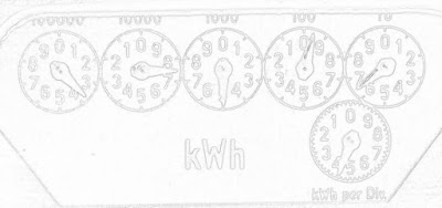
Finally the four corners are calculated separately, because each one has a unique combination of stencils required. Putting the loops in Fortran speeds things up considerably compared to the pure Python implementations I did before. Here is the gradient magnitude of the dials from Poor Man's ADC calculated with the above technique: