Uncertain Rate in FFT-based Oil Extraction Model

This is an extension to the FFT-based oil extraction model (see the Mobjectivist blog for more more details). The basic approach remains the same, each phase of the process is modeled by a convolution of the rate in the previous phase with an exponential decay. Now we are going to apply some of the ideas I presented in Uncertainty Quantification with Stochastic Collocation.

Here is the original Python function which applied the convolutions using an FFT,

 
def exponential_convolution(x, y, r): 
    """Convolve␣an␣exponential␣function␣e^(-r*x)␣with␣y,␣uses␣FFT.""" 
    expo = sp.exp(-r*x) 
    expo = expo / sp.sum(expo) # normalize 
    return(ifft(fft(expo) * fft(y)).real)

and here is the function modified to use the complex step derivative calculation method:

 
def expo_conv_csd(x, y, r): 
    """Convolve␣an␣exponential␣function␣e^(-r*x)␣with␣y,␣uses␣FFT.␣Use 
␣␣␣␣the␣complex␣step␣derivative␣method␣to␣estimate␣the␣slope␣with 
␣␣␣␣respect␣to␣the␣rate. 
 
␣␣␣␣See␣Cervino␣and␣Bewley,␣’On␣the␣extension␣of␣the␣complex-step 
␣␣␣␣derivative␣technique␣to␣pseudospectral␣algorithms’, 
␣␣␣␣J.Comp.Phys.␣187␣(2003). 
␣␣␣␣""" 
    expo = sp.exp(-r*x) 
    # normalize: 
    expo = expo / sp.sum(expo) 
    # need to transform the real and imag parts seperately to avoid 
    # problems due to subtractive cancellation: 
    expo.real = ifft(fft(expo.real) * fft(y)).real 
    expo.imag = ifft(fft(expo.imag) * fft(y)).real 
    return(expo)

Notice that we need to transform the real and imaginary parts of our solution separately so that the nice subtractive-cancellation-avoidance properties of the method are retained (see [1] for a more detailed discussion).

Now we have the result of the convolution in the real part of the return value and the sensitivity to changes in rate in the imaginary part (see Figure 1).

---

Figure 1: Rate sensitivity with a normally distributed input and normally distributed rate

---

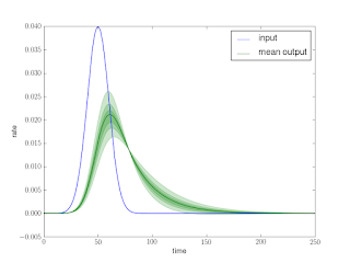
Now we proceed as shown before in the UQ post, except this time we have a separate probability density for the result at each time. Figure 2 shows the mean prediction as well as shading based on confidence intervals (at the 0.3, 0.6, and 0.9 level). The Python to generate this figure is shown below, it uses the alpha parameter (transparency) available in the matplotlib plotting package in a similar way to the vizualization approach shown in this post.

 
p.figure() 
p.plot(x, y, label="input") 
p.plot(x, y_mean, ’g’, label="mean␣output") 
p.fill_between(x, y_ci30[0], y_ci30[1], where=None, color=’g’, alpha=0.2) 
p.fill_between(x, y_ci60[0], y_ci60[1], where=None, color=’g’, alpha=0.2) 
p.fill_between(x, y_ci90[0], y_ci90[1], where=None, color=’g’, alpha=0.2) 
p.legend(loc=0) 
p.xlabel("time") 
p.ylabel("rate") 
p.savefig("uncertain_rate.png")

---

Figure 2: Results with an uncertain rate

---

Compare the result in Figure 2 with this Monte Carlo analysis. It’s not quite apples-to-apples, because that Monte Carlo includes uncertain discovery (the input) as well. Also, this result is just a first-order collocation, so it assumes that the rate sensitivity is constant with variations in the result. This is not actually the case, and you can see if you look closely that the 0.9-interval actually dips into negative territory, which is unphysical. This is a good example of the sort of common-sense checking Hamming suggested in his “N+1” essay as a requirement for any successful computation: Are the known conservation laws obeyed by the result? [2]. Clearly we are not going to “overshoot” on extraction and begin pumping oil back into the ground.

On a somewhat related note, Hamming had another insightful thing to say about the importance of checking the correctness of a calculation: It is the experience of the author that a good theoretician can account for almost anything produced, right or wrong, or at least he can waste a lot of time worrying about whether it is right or wrong [2]. Don’t worry,verify!

References

[1]   Cervino, L.I., Bewley, T.R., “On the extension of the complex-step derivative technique to pseudospectral algorithms,” Journal of Computational Physics, 187, 544-549, 2003.

[2]   Hamming, R.W., “Numerical Methods for Scientists and Engineers,” 2nd ed., Dover Publications, 1986.

(If you are serious about the art of scientific computing, that Dover edition of Hamming’s book is the best investment you could make with a very few bucks.)