I was putting together a little data post-processing tutorial for some guys in my lab, and it turned into a tour de force for that scientific computing swiss army knife, the FFT. So I figured I'd share it here.
The explicit recognition of its [the FFT’s] importance is one of the few significant advances in numerical
analysis in the past few decades. Much has been learned about various aspects of computation, but no other
recent discovery has so profoundly affected so many different fields as has the fast Fourier transform.
–R.W. Hamming [1]
This tutorial will demonstrate Gaussian convolution / deconvolution and Abel inversion of something resembling microwave interferometry data. The tutorial uses Scipy [2], but the concepts (as well as most of the function names and even the underlying FFT libraries) transfer directly to other environments (Matlab, Octave, etc). When in doubt, Google or Hutchinson [3] are your friends.
1 Gaussian Convolution / Deconvolution
The Microwave Interferometer beam is assumed to have a Gaussian distribution of intensity. The equation for a Gaussian distribution is
 | (1) |
This means that the measurement at each spatial position is a “mixture” of effects from neighboring areas along the beam’s axis. To understand this, we’ll do some convolutions with Gaussians. First off, we need an array of points
from a Gaussian, but we need them in a particular order. Here’s a Python function which does what we need:
def periodic_gaussian(x, sigma):
nx = len(x)
# put the peak in the middle of the array: mu = x[nx/2]
g = gaussian(x, mu, sigma)
# need to normalize, the discrete approximation will be a bit off: g = g / sum(g)
# reorder to split the peak across the boundaries: return(sp.append(g[nx/2:nx], g[0:nx/2]))
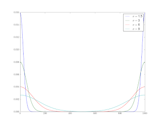
The reason for reordering is because we’ll be using FFTs to do the convolutions, and the FFT assumes periodic data. Figure 1 shows the results for several values of the standard deviation.
Once we have the proper distributions defined, the convolution just requires an FFT of the theoretical curve, and the Gaussians, point-wise multiplication in the transformed-domain, followed by an inverse transform. The Python to do this is shown below:
dx = x[1]
- x[0]
sigma = [25.0, 50.0, 100.0, 150.0]
g = []
cyl_conv = []
fcyl = fft(cyl)
for i,s
in enumerate(sigma):
g.append(periodic_gaussian(x, s
*dx))
cyl_conv.append(ifft(fcyl
* fft(g[i])))
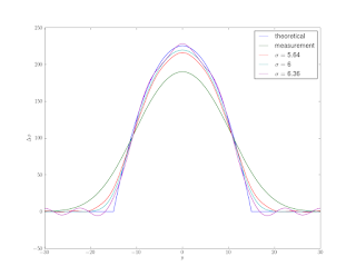
Figure 2 shows a theoretical phase shift curve for a calibration cylinder along with convolutions of that same curve with Gaussians of various standard deviations.
Convolution is easy enough, but what we have in the case of an interferometry measurement is the convolved signal, and we’d like the ’true’ measurement. We can get this by deconvolution. This is simply division in the frequency space as opposed to multiplication:
# now try a deconvolution: sigma_deconv = [94.0, 100.0, 106.0]
cyl_deconv = []
# use one of the previous convolutions as our ’measurement’: fmeas = fft(cyl_conv[2])
for i,s
in enumerate(sigma_deconv):
cyl_deconv.append(ifft(fmeas / fft(periodic_gaussian(x, s
*dx))))
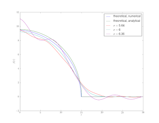
Figure 3 shows the results for a couple test σ’s. Unfortunately, deconvolution is numerically ill-posed and very sensitive to noise, it tends to amplify any noise present. Unless we are very lucky and guess the exact σ and our measurement has no noise, we end up with ’wiggles’.
We can fix things by first ’smoothing’ with a small Gaussian, and then performing some test deconvolutions.
# now try a deconvolution with some ’regularization’: sigma_reg = 50.0
# about half our ’true’ sigma cyl_deconv_smooth = []
# use one of the previous convolutions as our ’measurement’, smooth it: fmeas = fft(cyl_conv[2])
* fft(periodic_gaussian(x, sigma_reg
*dx))
for i,s
in enumerate(sigma_deconv):
cyl_deconv_smooth.append(ifft(fmeas / fft(periodic_gaussian(x, s
*dx))))
The deconvolution that uses σ > σtrue still displays overshoots even with the smoothing, it also becomes too ’sharp’. The calibration measurements can be used to find the optimal smoothing and sharpening σ for the particular interferometer / frequencies being used.
2 Abel Inversion
Many of the same tools presented in Section 1 can be extended to the calculation of the Abel inversion. In microwave interferometry we have a ’chord-averaged’ measurement, but we would like to understand the radial distribution of the quantity (phase shift / plasma density).
 | (2) |
where F is our chord-averaged measurement, and f(r) is the radial distribution that we would like to recover. To calculate the inverse transform we first need an estimate of the derivative ∂F∕∂y. Like deconvolution, numerical differentiation tends to amplify noise (numerical or otherwise). To avoid this we can convolve the derivative of a Gaussian with the function we wish to differentiate and then perform an inverse transform to recover a ’smoothed’ numerical derivative. The derivative of the Gaussian is
 | (3) |
A Python function that gives a properly re-ordered first derivative is
def periodic_gaussian_deriv(x, sigma):
nx = len(x)
# put the peak in the middle of the array: mu = x[nx/2]
g = dgaussiandx(x, mu, sigma)
# need to normalize, the discrete approximation will be a bit off: g = g / (
-sp.sum(x
* g))
# reorder to split the peak across the boundaries: return(sp.append(g[nx/2:nx], g[0:nx/2]))
In the same way that we used the Gaussian for smoothing we can use its derivative for differentiation. Here’s the Python to do that:
# calculate some derivatives: sigma_deriv = 0.5
# this can be small because we’ve already smoothed a lot cyl_deriv = []
for i,c
in enumerate(cyl_deconv_smooth):
cyl_deriv.append(
ifft(fft(c)
* fft(periodic_gaussian_deriv(x, sigma_deriv
*dx))).real)
Figure 5 shows the results. The wiggles that we don’t manage to smooth in the initial sharpening stage become amplified by differentiation.
Once we have a numerical approximation for the derivative, calculating the integral is straight-forward:
def abel(dfdx, x):
nx = len(x)
# do each half of the signal separately (they should be the same # up to noise) integral = sp.zeros((2,nx/2), dtype=float)
for i
in xrange(nx/2, nx
-1):
divisor = sp.sqrt(x[i:nx]
**2
- x[i]
**2)
integrand = dfdx[i:nx] / divisor
integrand[0] = integrand[1]
# deal with the singularity at x=r integral[0][i
-nx/2] =
- sp.trapz(integrand, x[i:nx]) / sp.pi
for i
in xrange(nx/2, 1,
-1):
divisor = sp.sqrt(x[i:0:
-1]
**2
- x[i]
**2)
integrand = dfdx[i:0:
-1] / divisor
integrand[0] = integrand[1]
# deal with the singularity at x=r integral[1][
-i+nx/2] =
- sp.trapz(integrand, x[i:0:
-1]) / sp.pi
return(integral)
The one minor ’gotcha’ is dealing with the integrable singularity in 2. We just copy the value of the nearest neighbor over the Inf, the integral will approach the correct value in the limit of small Δx (lots of points).
The analytical inverse Abel transform of the theoretical phase shift curve can be easily calculated (Maxima [4] script shown in section A.2). The theoretical phase shift has the form
 | (4) |
which gives the derivative as
 | (5) |
and finally, the inverse Abel transform as
 | (6) |
2.1 Centering
Often, despite our best efforts, the data are not centered. There is a method to estimate the optimal shift required to center the data using the FFT [5]. Figure 7 shows one of the “measurements” shifted by a small amount.
The method of Jaffe et al. [5] is to maximize
![N∕2-1 ∑ [ -2πmk Δfn ]2 Re(e Lnh) -N ∕2](https://blogger.googleusercontent.com/img/b/R29vZ2xl/AVvXsEgey9LM9xfdMaMFFvvbB04nDHSHO_-ExftZuSHvzZsFrCXgXiBtRokrFGpJWrcVxGiYDun0bgzrIN5JFgE6NqfwC5YrlTe1jB0mbBTlza_ON4ncYOieht3pjtMcpejqQI6FKsI5LHl_pLM/s320/abel6x.png) | (7) |
Where Lnh is the Fourier transform of the data, and mkΔ is a shift. Since the data is real, the real part of its transform is the even part of the signal. The shift which maximizes the magnitude of the even part is the one which makes the data most even (centered). A graphical analysis of the data can provide a range of shifts to try. The Python to perform this maximization is shown below (this relies on being able to index arrays with arrays of integers, which can be done in Matlab as well).
# a shifted measurement shift = nx / 10
# a ten percent shift cyl_shifted = cyl_conv[2][scipy.append(range(shift,nx), range(0,shift))]
# find the shift needed to center the measurement (should match shift above): indices = []
# get range of shifts to try from ’eye-balling’ the measurement try_shift = range(nx
- 2
*shift, nx)
for i
in try_shift:
indices.append(scipy.append(range(i,nx), range(0,i)).astype(int))
even_norm = sp.zeros(len(indices), dtype=float)
for i, cyclic_perm
in enumerate(indices):
even_norm[i] = sp.sum(fft(cyl_shifted[cyclic_perm]).real
**2)
max_even_shift = try_shift[even_norm.argmax()]
Figure 8 shows that the objective function (equation 7) reaches a local maximum at the shift which was originally applied (shown in Figure 7).
3 Calibration Model Fitting
The techniques presented in section 1 can be combined to fit a calibration model to interferometry measurements of a calibration cylinder (or any other object for which you have the theoretical phase-shift curve). The purpose of a calibration model is to provide estimates of parameters like the standard deviation of the Gaussian beam for use in deconvolution and inversion of subsequent test measurements.
There steps in fitting the model are
- Center the data (2.1)
- Find an error minimizing set of deconvolution and smoothing σs (these are the parameters of our model).
- Define a function of the data and the σs which returns an error norm between the theoretical phase shift curve and the smoothed, deconvolved data.
- Apply a minimization algorithm to this function. Choose an initial guess for the deconvolution σ which is likely to be smaller than the true σ.
The Python functions to accomplish this are shown below. One error function uses a sum of squared errors and the other uses a maximum error.
def smooth_deconv(s, x, data):
fsmooth = fft(data)
* fft(periodic_gaussian(x, s[0]))
fdeconv = ifft(fsmooth / fft(periodic_gaussian(x, s[1]))).real
return(fdeconv)
def cal_model_ls_err(s, x, data, theoretical):
fdeconv = smooth_deconv(s, x, data)
return(sp.sqrt(sp.sum((fdeconv
- theoretical)
**2)))
def cal_model_minmax_err(s, x, data, theoretical):
fdeconv = smooth_deconv(s, x, data)
return((abs(fdeconv
- theoretical)).max())
The error in the fitted model following this approach is shown in Figure 9. Both the least squares error and the min-max error methods recover the correct deconvolution σ.
4 Further Improvements / Variations
Jaffe et al. [5] also suggest “symmetrizing” before calculating the Abel transform by removing the imaginary component of the transformed data. They also estimate the variance of the inverse Abel transform based on both the portion of the data removed by filtering (smoothing) and symmetrizing.
Rather than calculating the derivative necessary for the inverse Abel transform with a convolution, a pseudo-spectral method could be used. The trade-off being that very accurate derivatives could be attained at the expense of greatly amplifying any noise. A more practical variation, that is not susceptible to noise, would be to calculate the integral with a pseudo-spectral approach rather than the composite trapezoidal rule. This would give a more accurate integral, and bring the numerical and analytical curves in Figure 6 into closer agreement.
A Complete Scripts
A.1 Python
The complete Python script to do all of the calculations and generate all of the plots in this tutorial is available.
A.2 Maxima
The Maxima batch file used to calculate the inverse Abel transform of the theoretical phase-shift curve is available.
References
[1] Hamming, R.W., “Numerical Methods for Scientists and Engineers ,” 2nd. ed., Dover Publications, 1986.
[2] Jones, E., Oliphant, T., Peterson, P., “Scipy: Open source scientific tools for Python,” 2001–,
http://www.scipy.org
[3] Hutchinson, I.H., “Principles of Plasma Diagnostics ,” 2nd ed., Cambridge University Press, 2002.
[4] Schelter, W., et al., “Maxima: a computer algebra system,” http://maxima.sourceforge.net
[5] Jaffe, S.M., Larjo, J., Henberg, R., “Abel Inversion Using the Fast Fourier Transform,” 10th International Symposium on Plasma Chemistry, Bochum, (1991).


![N∕2-1 ∑ [ -2πmk Δfn ]2 Re(e Lnh) -N ∕2](https://blogger.googleusercontent.com/img/b/R29vZ2xl/AVvXsEgey9LM9xfdMaMFFvvbB04nDHSHO_-ExftZuSHvzZsFrCXgXiBtRokrFGpJWrcVxGiYDun0bgzrIN5JFgE6NqfwC5YrlTe1jB0mbBTlza_ON4ncYOieht3pjtMcpejqQI6FKsI5LHl_pLM/s320/abel6x.png)


